Recursive functions
Recursive function body references the function itself. Such approach is used to describe in a more clear
and simple way the algorithmical problem which depends on solving smaller instances of the same problem.
In this article we present typical features of recursive functions with examples implemented in POOL.
- The factorial function
- Simple fractals
- Mutual recursion
- Fibonacci series
The factorial function
The factorial of a natural number n is calculated as a product of all natural numbers less than or equal
to n:
n! = 1 * 2 * 3 * ... * n, for example:
5! = 1 * 2 * 3 * 4 * 5 = 120. A recursive algorithm for the factorial calculation can be written as:
a) n! = n * (n - 1)! if n > 1
b) n! = 1 if n ≤ 1
Note: each recursive algorithm requires a stop condition. The above algorithm calculates the factorial
as a product of the number and the factorial of the number decreased by 1 (a). The sequence is stopped when the
algorithm reaches n = 1 and the stop condition (b) is fulfilled.
Recursive implementation of the factorial function in POOL is following:
to factorial :n
print :n
if :n <= 1 [output 1]
output :n * factorial :n - 1
end
(print ""|5! =| factorial 5)
The program result (in the text output window):
5
4
3
2
1
5! = 120
The factorial function has one argument, n, and returns the value of n!.
Syntax of the function definition was described in the previous chapter.
Here the conditional statement appears for the first time: if.
It allows to execute a block of code (here: output 1)
if the condition given as the first argument is met (here: :n <= 1).
The factorial function prints out the current value of :n on each execution to illustrate
the order of the function calls. Note that the instruction factorial 5 results with five executions of the
function that calls itself with argument values down to 1. An important feature of recursive funtions is
related to this behaviour: a copy of the function arguments and local variables is stored in the memory for each
recursive call of the function. The amount of memory required by the recursive algorithm implementation may become
significant, and eventually a non-recursive equivalent may be needed. In case of the factorial function it could be:
to factorial_1 :n
if :n <= 1 [output 1]
let "k :n
while :n > 2 [
"n := :n - 1
"k := :k * :n
]
output :k
end
The above function needs only two variables, the argument :n and the local variable :k
to calculate factorial of any value.
Simple fractals
Drawing of many fractals can be easyli programmed using recursive functions. They are figures, of which smaller
parts resemble the whole, which is the essence of recursion. The two examples below are taken from the
fractals, part I project.
The Koch Flake
Let's start from a simple function:
to k1 :r
fd :r/3 rt 60
fd :r/3 lt 120
fd :r/3 rt 60
fd :r/3
end
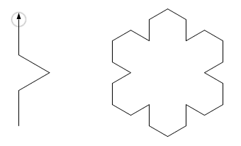
A single call to k1 draws a figure's one side with a size of :r, like on the left image.
A six-fold repetition with the rotation completes the figure, as shown on the right.
repeat 6 [k1 90 rt 60]
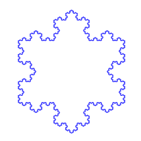
And now a small modification: each step fd :r/3
is substituted with the recursive call koch :r/3 :g-1,
which simultaneously decreases the counter :g; the stop condition is following:
:g = 0:
to koch :r :g
if :g = 0 [fd :r stop]
koch :r/3 :g-1 rt 60
koch :r/3 :g-1 lt 120
koch :r/3 :g-1 rt 60
koch :r/3 :g-1
end
repeat 6 [koch 90 5 rt 60]
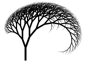
The Tree
The Tree belongs to another popular family of fractals. Various forms can be achieved by modification of the function below.
Also the fern leaves, which you can find in the project, fall in this cathegory
of fractals.
to tree :r :g
if :g > 0 [
setpensize :g
fd :r
lt 20
tree :r * 0.7 :g - 2
rt 40
tree :r * 0.9 :g - 1
lt 20
pu bk :r pd
]
end
tree 100 15
Mutual recursion
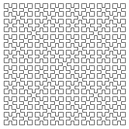
Also the two independent functions can call each other, as in the following example of the Wirth curve:
to wi :n :a :h :k
if :n = 0 [fd :h stop]
rt :a iw :n (-:a) :h :k lt :a fd :h
lt :a iw :n (-:a) :h :k rt :a
end
to iw :n :a :h :k
rt :a wi :n - 1 (-:a) :h :k fd :k lt 2 * :a
fd :k wi :n - 1 (-:a) :h :k rt :a
end
to wirth :n :s
repeat 4 [
wi :n 45 3*:s :s
fd :s rt 90 fd :s
]
end
wirth 4 2
Such mutually recursive algorithm can be transformed into a standard, single recursive function wi by
inlining calls to the iw function, however the resulting code is less elegant.
Mutual recursion is not very commonly used in practice, but one of the few good examples are
recursive descent parsers.
Fibonacci series
Another typical example is the recursive algorithm for the Fibonacci series calculation. Consecutive numbers in this
series are: f0 = 0, f1 = 1,
fn = fn-1 + fn-2.
A recursive function to calculate them can be:
to fibo_rec :n
if :n < 2 [output :n]
output (fibo_rec :n-2) + (fibo_rec :n-1)
end
Although the function itself is simple, the calculation time for n above 30-40 becomes noticeable... it is
due to the fact that the single call to the function triggers two recursive calls, which in turn recursively call the
function two more times each, and so on, up to the total number of 331160281 function calls for
n = 40. A non-recursive equivalent of the algorithm is very helpful in this case. Try the
following code:
to fibo_alg :n
if :n < 2 [output :n]
let "n2 0
let "n1 1
let "nx 0
repeat :n-1 [
"nx := :n2 + :n1
"n2 := :n1
"n1 := :nx
]
output :nx
end
The Fibonacci series, as every other series, whose elements are given with a linear combination of preceding
elements with constant coefficients, can be expressed with a formula for n-th element. Finally, such
calculation method is the most efficient:
to fibo_mat :n
output round ((0.5 * (1 + sqrt 5))^:n) / (sqrt 5)
end
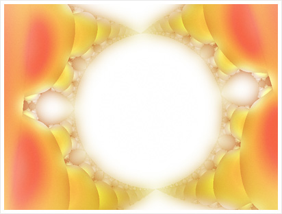
The Fibonacci series has a version generalized for the complex numbers. The series can be visualized on the
2D plane, coloured with the escape time algorithm, often used for fractals painting. An example of such
prepared image, also obtained with POOL code, is shown below. However this topic itself deserves a separate article.